My first simulation

As introduction to the gamdpy package let us setting up a simulation of a Lennard-Jones FCC crystal in the constant \(NVT\) ensemble. For a short summary, see the minimal.py example script. Also, the line sim = gp.get_default_simulation() will create a simulation object similar to the below.

If gamdpy is installed correctly, the following package should be imported without any errors. It is recommended to import the package as gp.

import gamdpy as gp

*We will also import NumPy for numerical calculations and Matplotlib for plotting.

import numpy as np  # For numerical operations
import matplotlib.pyplot as plt  # For plotting

Initial particle positions

We wish to set up a configuration of a FCC lattice with \(8 \times 8 \times 8\) unit cells, with a density of \(\rho = 0.973\). First we create an empty configuration object.

configuration = gp.Configuration(D=3)

Information for a few crystal unit cells are avalible with the gamdpy package. For example, the FCC unit cell is stored as rp.unit_cells.FCC.

gp.unit_cells.FCC

{'fractional_coordinates': [[0.0, 0.0, 0.0],
  [0.5, 0.5, 0.0],
  [0.5, 0.0, 0.5],
  [0.0, 0.5, 0.5]],
 'lattice_constants': [1.0, 1.0, 1.0]}

We use the make_lattice method to assign positions and a simulation box to the configuration object.

# Setup configuration: FCC Lattice
configuration.make_lattice(
    unit_cell=gp.unit_cells.FCC,
    cells=[8, 8, 8],
    rho=0.973
)

The positions can be accessed with ['r']. All vector properties, like the positions, are NumPy arrays.

positions = configuration['r']
type(positions)

numpy.ndarray

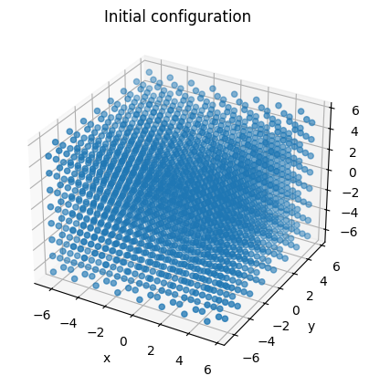
To confirm that the positions are as expected, we can visualize the configuration using Matplotlib.

# Make 3D plot using matplotlib
fig = plt.figure()
ax = fig.add_subplot(111, projection='3d')
ax.set_title('Initial configuration')
ax.scatter(positions[:,0], positions[:,1], positions[:,2])
ax.set_xlabel('x')
ax.set_ylabel('y')
ax.set_zlabel('z')
plt.show()

The configuration object also contains a simulation box. Here we use an orthorhombic box. The box lengths can be accessed as seen below.

configuration.simbox.get_lengths() # Box lengths

array([12.815602, 12.815602, 12.815602], dtype=float32)

Masses and initial velocities

We set all particle masses to one (the value is broadcast to all particles).

configuration['m'] = 1.0  # Set all masses to 1.0

Note that configuration['m'] refer to an NumPy array. For convenience, we above used a float to set all masses to the same value. This value will automatically be broadcast to all particles.

type(configuration['m'])  # configuration['m'] is a NumPy array

numpy.ndarray

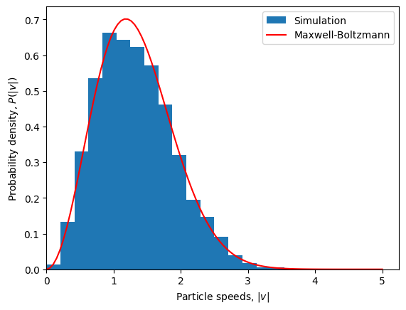
After masses are set, we can assign random velocities corresponding to an initial kinetic temperature \(T = 0.7\).

temperature = 0.7
configuration.randomize_velocities(temperature=temperature)

To confirm that the initial velocity distribution is as expected, we can compare it the the theoretical Maxwell-Boltzmann distribution.

plt.figure()
# Histogram of particle speeds
vel = configuration['v']
speeds = np.linalg.norm(vel, axis=1)
bins = np.linspace(0, 5, 25)
plt.hist(speeds, bins=bins, density=True, label='Simulation')
# Theoretical Maxwell-Boltzmann distribution
v = np.linspace(0, 5, 100)
maxwell_boltzmann = (2*np.pi*temperature)**(-3/2)*4*np.pi*v**2*np.exp(-v**2/(2*temperature))
plt.plot(v, maxwell_boltzmann, label='Maxwell-Boltzmann', color='r')
# Plot settings
plt.xlabel(r'Particle speeds, $|v|$')
plt.ylabel(r'Probability density, $P(|v|)$')
plt.xlim(0, None)
plt.legend()
plt.show()

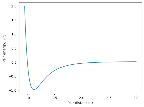
Pair potential

Next, we set up the Lennard-Jones pair potential. We use the 12-6 Lennard-Jones potential

\[ v_\infty(r) = 4\varepsilon \left[\left(\frac{\sigma}{r}\right)^{12} - \left(\frac{\sigma}{r}\right)^{6}\right] \]

(the substript refer to a “truncation” at \(\infty\)). Here \(\sigma\) (sigma) is length, and \(\varepsilon\) (epsilon) is an energy. We will use Lennard-Jones units, where \(\sigma = 1\) and \(\varepsilon = 1\).

Several pair potentials functions are implemented in gamdpy, and the above 12-6 Lennard-Jones potential is implemented as gp.LJ_12_6_sigma_epsilon. This is a Python function that takes distances, parameters as input and returns the potential energy, the force and the second derivative of the potential energy.

Let us confirm values are as expected in the minimum of the potential:

(1)\[\begin{align} r_{min} &= 2^{1/6} \\ v(r_{min}) &= -\varepsilon \\ f(r_{min}) &= 0 \\ \left.\frac{d^2v}{dr^2}\right|_{r_{min}} &= (624\cdot2^{-7/3}-168\cdot2^{-4/3})\frac{\varepsilon}{\sigma^2} \simeq 57.146\frac{\varepsilon}{\sigma^2} \end{align}\]

pair_func = gp.LJ_12_6_sigma_epsilon  # Pair potential function
r_min = 2**(1/6)
u_min, f_min, curvature_min = pair_func(r_min, (1.0, 1.0, np.inf))
u_min, f_min, curvature_min

(np.float32(-0.99999994), np.float32(-5.6769886e-07), np.float32(57.146423))

To allow for a \(O(N)\) algorithm for force calculations, we truncate the pair potential at radius of \(r_c = 2.5\sigma\) (cutoff). The potential is shifted to zero at the cutoff radius, so the actual potential is

\[ v(r) = v_\infty(r) - v_\infty(r_c) \]

For this, we can use gp.apply_shifted_potential_cutoff to modify the pair potential.

pair_func = gp.apply_shifted_potential_cutoff(gp.LJ_12_6_sigma_epsilon)

Let us plot the pair potential, so confirm that it looks as we expect.

sigma, epsilon, cutoff = 1.0, 1.0, 2.5
pair_distances = np.linspace(0.95, 3.0, 128)
pair_energies = [pair_func(dist, [sigma, epsilon, cutoff])[0] for dist in pair_distances]

plt.figure()
plt.plot(pair_distances, pair_energies)
plt.xlabel(r'Pair distance, r')
plt.ylabel(r'Pair energy, $v(r)$')
plt.show()

We can now create an interaction objects using this pair potential function we made.

pair_pot = gp.PairPotential(pair_func, params=[sigma, epsilon, cutoff], max_num_nbs=1000)

Finally, we create a list will all the interactions in our simulations. In this simulation, we only have one, but later we may want to include more like bonds, walls, or gravity.

interactions = [pair_pot, ]

Integrator

Next, create an integrator object. These are available in the submodule gamdpy.integrators. Here, we chose to use and implementation of the Nosé-Hoover thermostat discretion using the Leap-Frog scheme (others are available). We set a time-step of \(dt=0.005\) and a thermostat relaxation time to \(\tau = 0.2\) (both in Lennard-Jones units).

# Setup integrator: Nosé-Hoover NVT, Leap-frog algorithm
integrator = gp.integrators.NVT(temperature=temperature, tau=0.2, dt=0.005)

Runtime actions

We typically wants to do some actions during the simulations. Below we specify that we want to store configurations (particle positions, velocities, …).

• The gp.TrajectorySaver does this using a logarithmic timescale in each timeblock.

• The gp.ScalarSaver save scalar properties like energy every steps_between_output=16 timestep.

• During long-time simulations, there might be a drift of the total momentum due to floating point rounding erros. Thus, the gp.MomentumReset reset the total momentum every steps_between_reset=100 timestep. All the runtime actions are collected in a list.

steps_between_output = 16
runtime_actions = [
    gp.TrajectorySaver(),
    gp.ScalarSaver(steps_between_output=steps_between_output),
    gp.MomentumReset(steps_between_reset=100),
]

The Simulation object

We now have all the components to set up a simulation object.

• An configuration object (particle positions, velocities, masses, …).

• A list of interactions (here the Lennard-Jones potential).

• An integrator object (here the Nosé-Hoover thermostat).

• A list of runtime actions

For the simulation object we also specify that we want num_timeblocks=32 time blocks of steps_per_timeblock=1024 steps. We also specify that we want to store the simulation data in a file with storage='LJ_T0.70.h5'. Change to storage='memory' if you do not want to save a file to the disk.

# Setup Simulation
sim = gp.Simulation(configuration, interactions, integrator, runtime_actions,
                    num_timeblocks=32,
                    steps_per_timeblock=1024,
                    storage='LJ_T0.70.h5')

Running the simulation

Finally, we run the simulation using the sim.run_timeblocs iterator that will loop over all the timeblocs. Below we print the status of the simulation after each timeblock.

for timeblock in sim.run_timeblocks():
        print(sim.status(per_particle=True))
print(sim.summary())

timeblock= 0     time= 5.120       U= -6.256    W= 0.885     K= 1.053     
timeblock= 1     time= 10.240      U= -6.310    W= 0.590     K= 1.058     
timeblock= 2     time= 15.360      U= -6.294    W= 0.669     K= 1.045     
timeblock= 3     time= 20.480      U= -6.314    W= 0.563     K= 1.032     
timeblock= 4     time= 25.600      U= -6.292    W= 0.685     K= 1.073     
timeblock= 5     time= 30.720      U= -6.262    W= 0.847     K= 1.007     
timeblock= 6     time= 35.840      U= -6.329    W= 0.480     K= 1.033     
timeblock= 7     time= 40.960      U= -6.309    W= 0.586     K= 1.030     
timeblock= 8     time= 46.080      U= -6.273    W= 0.789     K= 1.033     
timeblock= 9     time= 51.200      U= -6.279    W= 0.749     K= 1.048     
timeblock= 10    time= 56.320      U= -6.295    W= 0.663     K= 1.029     
timeblock= 11    time= 61.440      U= -6.278    W= 0.763     K= 1.060     
timeblock= 12    time= 66.560      U= -6.265    W= 0.830     K= 1.015     
timeblock= 13    time= 71.680      U= -6.267    W= 0.835     K= 1.043     
timeblock= 14    time= 76.800      U= -6.276    W= 0.760     K= 1.039     
timeblock= 15    time= 81.920      U= -6.303    W= 0.610     K= 1.034     
timeblock= 16    time= 87.040      U= -6.307    W= 0.585     K= 1.053     
timeblock= 17    time= 92.160      U= -6.271    W= 0.811     K= 1.057     
timeblock= 18    time= 97.280      U= -6.308    W= 0.580     K= 1.040     
timeblock= 19    time= 102.400     U= -6.275    W= 0.776     K= 1.058     
timeblock= 20    time= 107.520     U= -6.303    W= 0.639     K= 1.048     
timeblock= 21    time= 112.640     U= -6.274    W= 0.794     K= 1.054     
timeblock= 22    time= 117.760     U= -6.274    W= 0.798     K= 1.075     
timeblock= 23    time= 122.880     U= -6.306    W= 0.583     K= 1.049     
timeblock= 24    time= 128.000     U= -6.300    W= 0.637     K= 1.048     
timeblock= 25    time= 133.120     U= -6.271    W= 0.783     K= 1.058     
timeblock= 26    time= 138.240     U= -6.313    W= 0.571     K= 1.053     
timeblock= 27    time= 143.360     U= -6.293    W= 0.665     K= 1.029     
timeblock= 28    time= 148.480     U= -6.270    W= 0.799     K= 1.041     
timeblock= 29    time= 153.600     U= -6.292    W= 0.685     K= 1.042     
timeblock= 30    time= 158.720     U= -6.279    W= 0.743     K= 1.028     
timeblock= 31    time= 163.840     U= -6.264    W= 0.846     K= 1.046     
Particles : 2048 
Steps : 32 * 1024 = 32_768 
Total run time  (incl. time spent between timeblocks): 1.37 s ( TPS: 2.39e+04 )
Simulation time (excl. time spent between timeblocks): 1.17 s ( TPS: 2.80e+04 )

The sim.status() and sim.summary() methods prints some basic information.

Analysis of data in memory

Simulation data, also written to the *.h5 file, is stored in memory and is accecible in sim.output:

output = sim.output  # Data stored in memory

Below, we extract some thermodynamic quantities stored in the simulation object.

# Extract potential energy, virial and kinetic energy
U, W, K = gp.extract_scalars(output, ['U', 'W', 'K'])
type(U)

numpy.ndarray

The variables U, W and K are NumPy arrays with the potential energy, virial and kinetic energy, respectively, for selected timesteps. The number of stored timestep can be found with len(U).

len(U)

2048

Below we compute the times related to when the scalar quantities were stored (in Lennard-Jones units).

dt = output.attrs['dt']  # Time-step for integrator
time = np.arange(len(U)) * dt * output['scalar_saver'].attrs['steps_between_output']

We can use Matplotlib to plot the potential energy per particle as a function of time. We use sim.configuration.N to get the number of particles.

N = sim.configuration.N  # Number of particles

plt.figure()
plt.plot(time, U/N)
plt.xlabel(r'Time, $t$ [$\sigma\sqrt{m/\varepsilon}$]')  # Time in LJ units
plt.ylabel(r'Potential energy per particle, $U$ [$\varepsilon$]')  # Energy in LJ units
plt.xlim(0, None)
plt.show()

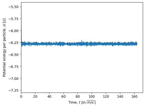
The first part of the simulation show large fluctuations in the potential energy since the system is not yet equilibrated (it was setup in a perfect crystal). Since we are not interested in the equilibration phase, we can discard the fir st timeblock by using the first_block=1 argument in the extract_scalars function. We then need to recalculate the time array.

U, W, K = gp.extract_scalars(sim.output, ['U', 'W', 'K'], first_block=1)
time = np.arange(len(U)) * dt * steps_between_output

plt.figure()
plt.plot(time, U/N, label='Potential energy per particle')
plt.xlabel(r'Time, $t$ [$\sigma\sqrt{m/\varepsilon}$]')  # Time in LJ units
plt.ylabel(r'Energy [$\varepsilon$]')  # Energy in LJ units
plt.legend()
plt.show()

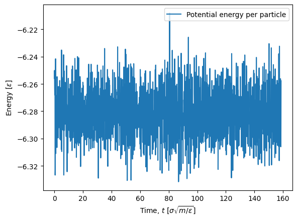
After we have ensured that we have an equilibrium simulation, the expectation value of the potential energy per particle can be found with the np.mean NumPy function.

np.mean(U/N)

np.float32(-6.281101)

In an \(NVT\) simulation the pressure is often an important quantity, but is not stored in the simulation data directly. The pressure can be calculated from the virial, \(W\). Recall,

\[ pV = Nk_BT + W \]

where \(p\) is the pressure, \(V\) is the volume, \(N\) is the number of particles, \(k\) is the Boltzmann constant and \(T\) is the temperature. The volume can be calculated from the box lengths. In Lennard-Jones units boltzmann constant is \(k_B = 1\). Below we use this to calculate the pressure.

V = sim.configuration.get_volume()  # Volume
dof = 3*N - 3  # Degrees of freedom
T_kin = 2*K/dof  # Kinetic temperature
p = (N*T_kin + W)/V  # Pressure
np.mean(p)  # Mean pressure

np.float32(1.4027747)

Concluding remarks

Congratulations! You have now set up and executed your first simulation with gamdpy. Simulation data have been stored to the disk for later analysis.