Post-run analysis

In the last tutorial, we simulated a Lennard-Jones crystal and stored data in the file 'LJ_T0.70.h5'. In this tutorial, we will analyse this data. Below, we will do some standard imports and load the data from the file on the disk.

# Imports
import numpy as np
import matplotlib.pyplot as plt
import h5py

import gamdpy as gp

# Select h5 file
filename='./LJ_T0.70.h5'
output = gp.tools.TrajectoryIO(filename).get_h5()

Found .h5 file (./LJ_T0.70.h5), loading to gamdpy as output dictionary

Brief about the h5 data file

Large data sets

Large data sets, such as the trajectory of particle positions, are stored as an HDF5 dataset (a data structure similar to a NumPy array, but data is stored on the disk).

nblocks, nconfs, N, D = output['trajectory_saver/positions'].shape
print(f'Number of timeblocks:          {nblocks = }')
print(f'Configurations per timeblock:  {nconfs = }')
print(f'Number of particles:           {N = }')
print(f'Number of spatial dimensions:  {D = }')

Number of timeblocks:          nblocks = 32
Configurations per timeblock:  nconfs = 12
Number of particles:           N = 2048
Number of spatial dimensions:  D = 3

Information in attributes

Some information, such as details about the simulation box, is stored as attributes. Below, we fetch such data to get the density of the NVT simulation.

simbox = output['initial_configuration'].attrs['simbox_data']
volume = np.prod(simbox)
rho = N/volume
print(f'Density:  {rho = }')

Density:  rho = np.float32(0.97300005)

Thermodynamics

The gamdpy package contains helper functions to read data in .h5 files. Thermodynamic data, stored in the 'scalar_saver' group, can be extracted using the gp.extract_scalars() function (we skip the first block with first_block=1 since the system is not equilibrated).

# Extract thermodynamic data
U, W, K = gp.extract_scalars(output, ['U', 'W', 'K'], first_block=1)

# Get times
dt = output.attrs['dt']  # Timestep
time = np.arange(len(U)) * dt * output['scalar_saver'].attrs['steps_between_output']

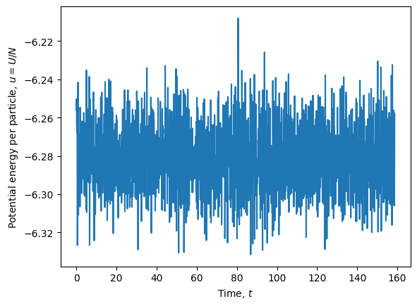
# Plot potential energy per particle as a function of time
plt.figure()
plt.plot(time, U/N)
plt.xlabel(r'Time, $t$')
plt.ylabel('Potential energy per particle, $u=U/N$')
plt.show()

Some properties need to be computed from the data stored. Examples are the kinetic temperature and pressure (in LJ units).

# Compute instantaneous kinetic temperature
dof = D * N - D  # degrees of freedom
T_kin = 2 * K / dof

# Compute instantaneous pressure
P = rho * T_kin + W / volume

print(f'Mean kinetic temperature:  {np.mean(T_kin) = }')
print(f'Mean pressure:             {np.mean(P) = }')

Mean kinetic temperature:  np.mean(T_kin) = np.float32(0.699899)
Mean pressure:             np.mean(P) = np.float32(1.4027747)

Structure

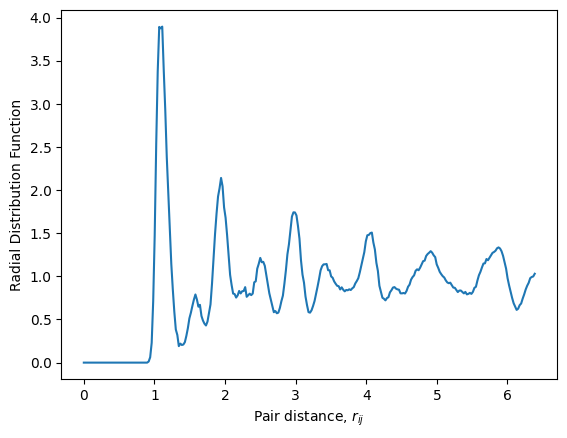
To investigate the structure and dynamics of particles, we need to analyse data in the 'trajectory_saver' group. Again, gamdpy has some built-in functionality to compute various measures. Let us calculate the radial distribution function. We will do this by inserting positions into a configuration object, and using the gamdpy.CalculatorRadialDistribution() class. The calculation is done on the GPU (for efficency).

# Create configuration object
configuration = gp.Configuration(D=D, N=N)
configuration.simbox = gp.Orthorhombic(D, output['initial_configuration'].attrs['simbox_data'])
configuration.ptype = output['initial_configuration/ptype']
configuration.copy_to_device()

# Call the radial distribution (RDF) calculator
calc_rdf = gp.CalculatorRadialDistribution(configuration, bins=300)

# Loop positions and compute the RDF
positions = output['trajectory_saver/positions'][:,:,:,:]
positions = positions.reshape(nblocks*nconfs,N,D)

# Loop over the last configurations in each time block
skipped_timeblocks = 1
start = nconfs-1+skipped_timeblocks*nconfs
step = nconfs
for pos in positions[start::step]:
    configuration['r'] = pos
    configuration.copy_to_device()
    calc_rdf.update()
rdf_data = calc_rdf.read()

# Plot RDF
plt.figure()
plt.plot(rdf_data['distances'], rdf_data['rdf'][0])
plt.xlabel(r'Pair distance, $r_{ij}$')
plt.ylabel('Radial Distribution Function')
plt.savefig(filename+'_rdf.pdf')
plt.show()

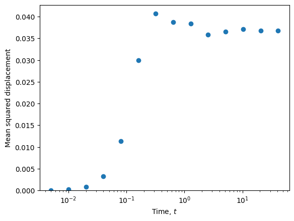
Dynamics

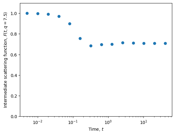
There are also built-in tools for analysing the trajectory. For example, the gamdpy.tools.calc_dynamics function computes several dynamical measures, including the mean squared displacement and the intermediate scattering function.

qvalues = 7.5
dynamics = gp.tools.calc_dynamics(output, first_block=1, qvalues=qvalues)  # Dictionary with dynamics
dynamics.keys()

dict_keys(['times', 'msd', 'alpha2', 'qvalues', 'Fs', 'count'])

plt.figure()
plt.plot(dynamics['times'], dynamics['msd'], 'o')
plt.xscale('log')
plt.ylim(0, None)
plt.xlabel(r'Time, $t$')
plt.ylabel(r'Mean squared displacement')
plt.show()

plt.figure()
plt.plot(dynamics['times'], dynamics['Fs'], 'o')
plt.xscale('log')
plt.ylim(0, 1.1)
plt.xlabel(r'Time, $t$')
plt.ylabel(r'Intermediate scattering function, $F(t, q = ' f'{qvalues}' r'$)')
plt.show()

Details about stored data

Structure of h5 file

Below is a function to print the structure of a given h5 file.

gp.tools.print_h5_structure(output)

initial_configuration/ (Group)
    ptype  (Dataset, shape=(2048,), dtype=int32)
    r_im  (Dataset, shape=(2048, 3), dtype=int32)
    scalars  (Dataset, shape=(2048, 4), dtype=float32)
    topology/ (Group)
        angles  (Dataset, shape=(0,), dtype=int32)
        bonds  (Dataset, shape=(0,), dtype=int32)
        dihedrals  (Dataset, shape=(0,), dtype=int32)
        molecules/ (Group)
    vectors  (Dataset, shape=(3, 2048, 3), dtype=float32)
scalar_saver/ (Group)
    scalars  (Dataset, shape=(32, 64, 3), dtype=float32)
trajectory_saver/ (Group)
    images  (Dataset, shape=(32, 12, 2048, 3), dtype=int32)
    positions  (Dataset, shape=(32, 12, 2048, 3), dtype=float32)

Attributes inside the H5 file

Below is a function that will print the attributes in a given h5 file.

gp.tools.print_h5_attributes(output)

Attributes at /:
    - dt: 0.005
    - script_content: ...
    - script_name: ...
Attributes at /initial_configuration/:
    - simbox_data: [12.815602 12.815602 12.815602]
    - simbox_name: Orthorhombic
Attributes at /initial_configuration/scalars:
    - scalar_columns: ['U' 'W' 'K' 'm']
Attributes at /initial_configuration/topology/molecules/:
    - names: []
Attributes at /initial_configuration/vectors:
    - vector_columns: ['r' 'v' 'f']
Attributes at /scalar_saver/:
    - scalar_names: ['U' 'W' 'K']
    - steps_between_output: 16

Concluding remarks

You have now conducted your first simulation and done some post-analysis of the trajectory. You now understand the basics of how gamdpy works, and are ready for more advanced simulations and analysis - see examples.